Predict marginal cumulative incidences with confidence intervals for a target trial population

Usage

predict(object, ...)

# S4 method for class 'trial_sequence_ITT'
predict(
  object,
  newdata,
  predict_times,
  conf_int = TRUE,
  ci_type = "sandwich",
  samples = 100,
  type = c("cum_inc", "survival")
)

# S4 method for class 'trial_sequence_PP'
predict(
  object,
  newdata,
  predict_times,
  conf_int = TRUE,
  samples = 100,
  ci_type = c("sandwich", "Nonpara. bootstrap", "LEF outcome", "LEF both",
    "Jackknife Wald", "Jackknife MVN"),
  type = c("cum_inc", "survival")
)

# S3 method for class 'TE_msm'
predict(
  object,
  newdata,
  predict_times,
  conf_int = TRUE,
  samples = 100,
  type = c("cum_inc", "survival"),
  ...
)

Arguments

object

Object from trial_msm() or initiators() or trial_sequence.

...

Further arguments passed to or from other methods.

newdata

Baseline trial data that characterise the target trial population that marginal cumulative incidences or survival probabilities are predicted for. newdata must have the same columns and formats of variables as in the fitted marginal structural model specified in trial_msm() or initiators(). If newdata contains rows with followup_time > 0 these will be removed.

predict_times

Specify the follow-up visits/times where the marginal cumulative incidences or survival probabilities are predicted.

conf_int

Construct the point-wise 95-percent confidence intervals of cumulative incidences for the target trial population under treatment and non-treatment and their differences. The default confidence interval construction methods simulates the parameters in the marginal structural model from a multivariate normal distribution with the mean equal to the marginal structural model parameter estimates and the variance equal to the estimated robust covariance matrix.

ci_type

Specify the method used to construct the confidence interval for a per-protocol estimand (estimand_type = "PP") (only available for trial_sequence object). 'sandwich': using the estimated robust sandwich covariance matrix; 'Nonpara. bootstrap', 'LEF outcome', 'LEF both', 'Jackknife Wald', 'Jackknife MVN'

samples

Number of samples used to construct the simulation-based confidence intervals.

type

Specify cumulative incidences or survival probabilities to be predicted. Either cumulative incidence ("cum_inc") or survival probability ("survival").

Value

A list of three data frames containing the cumulative incidences for each of the assigned treatment options (treatment and non-treatment) and the difference between them.

Details

This function predicts the marginal cumulative incidences when a target trial population receives either the treatment or non-treatment at baseline (for an intention-to-treat analysis) or either sustained treatment or sustained non-treatment (for a per-protocol analysis). The difference between these cumulative incidences is the estimated causal effect of treatment. Currently, the predict function only provides marginal intention-to-treat and per-protocol effects, therefore it is only valid when estimand_type = "ITT" or estimand_type = "PP".

The width of the confidence intervals for resampling-based methods ('Nonpara. bootstrap', 'LEF outcome', 'LEF both', 'Jackknife Wald') is determined by the presence of an id column in newdata. If included, the function accounts for sampling variation in the target population, which typically yields wider intervals. If omitted, the target population is treated as a fixed group, and the intervals reflect only the uncertainty from the original source model.

Examples

# Prediction for initiators() or trial_msm() objects -----

# If necessary set the number of `data.table` threads
data.table::setDTthreads(2)

data("te_model_ex")
predicted_ci <- predict(te_model_ex, predict_times = 0:30, samples = 10)

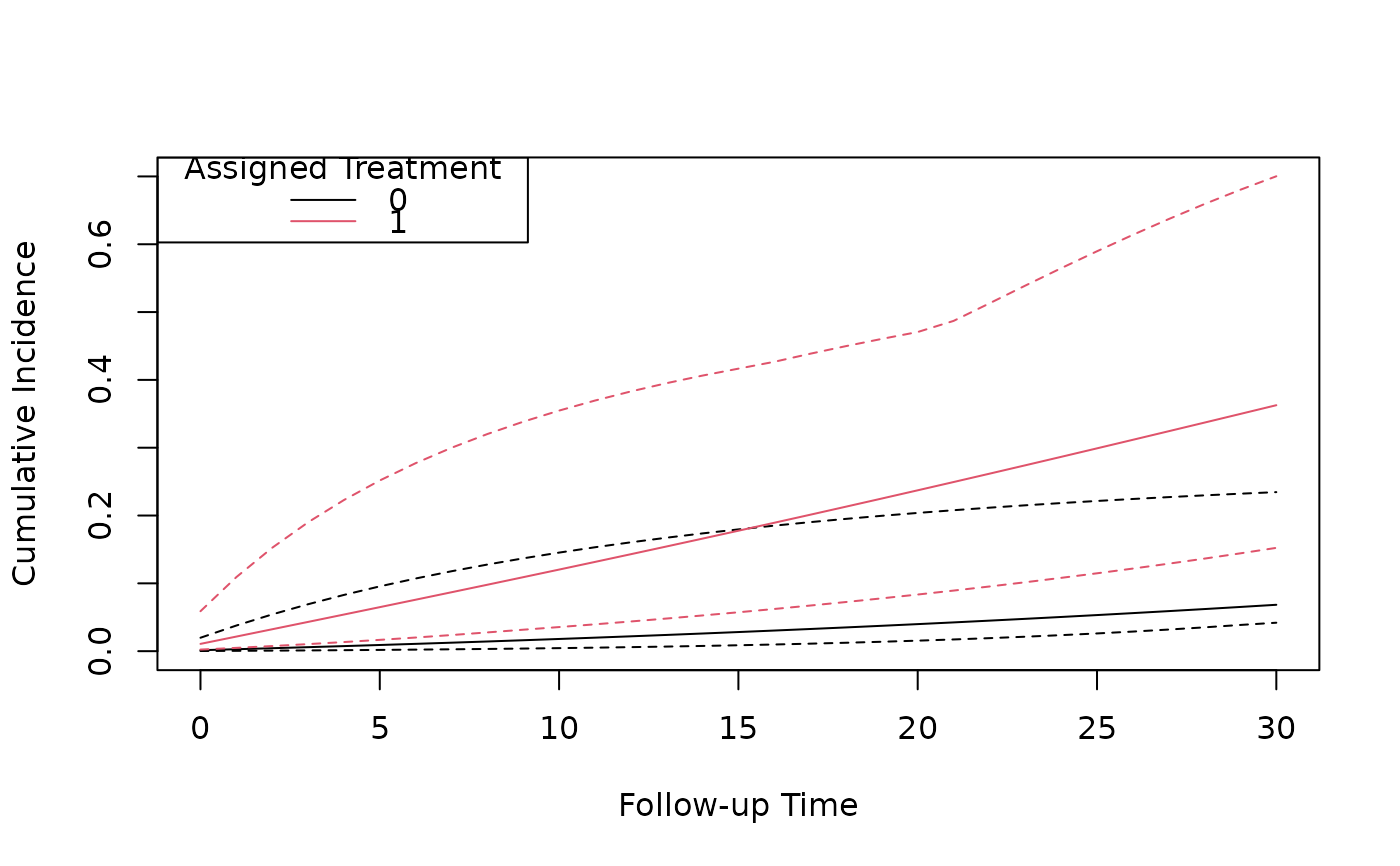
# Plot the cumulative incidence curves under treatment and non-treatment
plot(predicted_ci[[1]]$followup_time, predicted_ci[[1]]$cum_inc,
  type = "l",
  xlab = "Follow-up Time", ylab = "Cumulative Incidence",
  ylim = c(0, 0.7)
)
lines(predicted_ci[[1]]$followup_time, predicted_ci[[1]]$`2.5%`, lty = 2)
lines(predicted_ci[[1]]$followup_time, predicted_ci[[1]]$`97.5%`, lty = 2)

lines(predicted_ci[[2]]$followup_time, predicted_ci[[2]]$cum_inc, type = "l", col = 2)
lines(predicted_ci[[2]]$followup_time, predicted_ci[[2]]$`2.5%`, lty = 2, col = 2)
lines(predicted_ci[[2]]$followup_time, predicted_ci[[2]]$`97.5%`, lty = 2, col = 2)
legend("topleft", title = "Assigned Treatment", legend = c("0", "1"), col = 1:2, lty = 1)


# Plot the difference in cumulative incidence over follow up
plot(predicted_ci[[3]]$followup_time, predicted_ci[[3]]$cum_inc_diff,
  type = "l",
  xlab = "Follow-up Time", ylab = "Difference in Cumulative Incidence",
  ylim = c(0.0, 0.5)
)
lines(predicted_ci[[3]]$followup_time, predicted_ci[[3]]$`2.5%`, lty = 2)
lines(predicted_ci[[3]]$followup_time, predicted_ci[[3]]$`97.5%`, lty = 2)